The stopwatch study is one of the oldest instruments in industrial engineering, and everyone who has run one knows its two dirty secrets. The first is the sample: a study covers a few hours of a few shifts, chosen for when the engineer was available rather than when the process was interesting, and the standard it produces then governs planning for months of operation the study never saw. The second is the observer effect, which every operator can describe with a smile: work performed while an engineer stands beside the station with a clipboard is simply not the same work, and both parties know it. Continuous improvement has lived with these limits for a century because there was no alternative, and the honest name for much of what gets called cycle-time data is cycle-time estimate, extrapolated from moments nobody can prove were representative. This article is about what changes when the measurement runs continuously, from cameras already watching the line, and it builds on our pillar guide to AI-powered video analytics for manufacturing.
How continuous measurement works
Cycle-time analysis from video is one of the genuinely proven manufacturing applications of trained detection, delivered in real deployments alongside unit-flow tracking, and its mechanics are worth understanding because they explain both its power and its boundaries.
The foundation is the same detection-and-tracking stack described across this series: detection types trained on the plant's own footage recognize units and work states, tracking holds identity across frames so one unit is one object, and zone geometry drawn on each camera's view converts positions into process meaning. A station's cycle becomes measurable as the interval between a unit entering its zone and leaving it. Waiting becomes measurable as dwell in a queue zone. Utilization becomes measurable as the proportion of time a station zone contains active work. Flow between stations becomes measurable as transit intervals across zones, and material starvation shows up as the empty zone that should not be empty. None of these are exotic detections; they are ordinary events, read against geometry, accumulated forever.
Two properties separate this from every study that preceded it. Completeness: every cycle is measured, on every shift, through changeovers, through the difficult Stock-Keeping Unit (SKU), through the Friday afternoon nobody studies, which means the data contains the variance rather than an average that laundered it away. And invisibility: the measurement changes nothing on the floor, no clipboard, no observer, no altered behavior, so what accumulates is the process as it actually runs. The distribution that results is routinely a revelation on first viewing, not because the mean differs from the study, though it usually does, but because the shape of the variance was never visible before: the bimodal cycle that reveals two informal methods in use on different shifts, the long tail of interventions, the slow drift across a shift that no eight-cycle sample could catch.
How to read the distributions
The first continuous cycle-time distribution a team pulls tends to produce a silence, because nobody has seen their process drawn honestly before. Reading it is a skill worth naming, and three shapes carry most of the diagnostic weight.
A bimodal distribution, two humps where the standard assumed one, almost always means two methods in live use: day shift works the station one way, nights another, or two operators learned different sequences from different trainers. The stopwatch study captured whichever method happened to be running and called it the process. The distribution shows both, sized by frequency, and the CI conversation it triggers, which method is better and why has nobody standardized it, is usually worth more than the measurement program's first year of cost.
A long right tail, most cycles near standard with a scatter of multiples, is the signature of intervention: the cycles that included a jam clear, a missing tool hunt, a material wait. The tail's area is capacity being spent on friction, and each tail event has a timestamped clip behind it, which converts the tail from a statistical artifact into a reviewable list of specific frictions, rankable by frequency and cost.
And a drift, the distribution's center migrating across a shift, points at fatigue, heat, tool wear, or material behavior changing with time, each with its own remedy. Drift is invisible to any sampled study by construction, and it is the pattern operators have always described and never been able to prove.
Measuring changeovers
The same zone logic that times cycles times changeovers, and this may be where continuous measurement pays fastest in mixed-SKU plants. A changeover is an interval between the last good unit of one SKU and the first good unit of the next, and its official duration is typically a planning estimate defended by nobody. Zone events measure it as run: when flow actually stopped, how long each phase of the swap occupied the stations, when flow genuinely resumed, including the ragged restart period that estimates always exclude. Against that record, the classic Single-Minute Exchange of Die (SMED) questions, what was internal that could have been external, where did the crew wait on a crane, a part, a signoff, stop being workshop hypotheticals and become clip-backed observations from the last twenty real changeovers. Plants running this analysis consistently find the true changeover cost differs from the planned one by enough to change scheduling decisions, and the verification loop, measure, improve, keep measuring, holds the gains in a way workshop-week enthusiasm never has.
Finding the real bottleneck
Ask three supervisors where the constraint is and receive three confident answers, each anchored in memorable incidents rather than measurements. The stakes of guessing wrong are structural: improvement effort aimed anywhere but the constraint produces, by the standard logic of flow, precisely nothing at the system level, so the identification question is the most expensive one a CI program answers.
Continuous zone data answers it the way theory always said it should be answered: the constraint is where the queue persistently accumulates and downstream persistently starves, visible as dwell-time distributions by station across weeks of real mixed production rather than an afternoon of observation. What the continuous record adds beyond the textbook is the phenomenon plants actually live with, the wandering bottleneck. Constraints migrate with product mix, staffing, and the state of maintenance, and a study catches wherever the constraint happened to be that day, while the continuous record shows the migration itself: the wrapper constrains on SKU A, the palletizer on SKU B, and the whole system on Mondays because the weekend material staging runs late. That picture, constraint as a schedule rather than a place, is not obtainable any other way at reasonable cost, and it redirects improvement spending from the station with the loudest reputation to the pattern that actually governs output.
The verification loop closes the same way it does everywhere in this series: after the change, the same zones keep measuring, and the before-and-after distributions either show the improvement or they do not. A kaizen event whose result is a permanent measurement rather than a follow-up study six months later is a different kind of kaizen, and the discipline of confirming impact against continuous data, rather than declaring victory at the report-out, is quietly transformative for a CI program's credibility with plant leadership.
Measure the process, not the people
A capability this granular arrives with an obvious temptation, and the successful deployments name it early and refuse it in writing: this is process measurement, not people measurement. The distinction is technically real, cycles, queues, and utilization are properties of stations and flow, measurable on anonymous detections without identifying anyone, and it is operationally essential, because a workforce that believes the cameras are timing individuals will treat the system as the enemy it would in fact be, and the data will curdle alongside the trust.
The commitments that keep a CI deployment on the right side are the same package the safety articles in this series develop in full, and they transfer without modification: measurement of conditions and flow rather than individuals, no identification for process use cases, aggregate data shared with the workforce, and the no-discipline commitment in writing, works-council-agreed where applicable, covered in depth in our article on worker privacy and the no-discipline commitment. CI programs have one advantage here that safety programs lack: the improvement tradition already carries the right philosophy, that variance is a property of the process rather than a fault of the person, and a rollout that frames continuous measurement as the fulfillment of that philosophy, the end of blaming operators for what the stopwatch could not see, tends to land with the workforce as relief rather than surveillance. Operators, it turns out, have always known the standard was built on an unrepresentative afternoon, and a measurement that finally captures the Tuesday reality they actually work is a measurement many of them will defend.
There is also a practical honesty owed about what video measurement cannot see. Work inside machine enclosures, cognitive tasks, and micro-motions below camera resolution stay outside its reach, so the classic detailed time study retains its place for station-level method work. The continuous layer replaces the sampling problem, not the industrial engineer.
Start with one line
The failed version of this project tries to instrument everything and drowns in training and tuning before producing a single insight. The version that works picks one flow with a real question attached: the line whose output misses plan for reasons nobody agrees on, the cell whose standard everyone privately disbelieves.
The sequence is familiar from every deployment article in this series because it is the same sequence. Verify the cameras actually see the zones that matter, and move the one or two that do not, which is routine and cheap during planning and painful after. Train the unit and machine-state detection types on representative footage covering the real product mix, not the clean demo SKU. Run silent for two weeks to accumulate the baseline distribution before anyone reacts to it. Then read the data with the people who own the line, because the first review reliably surfaces context no engineer could infer alone, the informal second method, the known-bad fixture, the material issue everyone works around, and the measurement program's credibility is built or lost in whether that local knowledge is treated as correction or as excuse.
From there the cadence is the CI program's own: the continuous distributions feed the existing improvement pipeline, constraint identification stops being an argument, and every implemented change gets its verification chart from the zones that never stopped watching.
A word on where this data should live organizationally: with the CI function, not with supervision. The distributions are diagnostic instruments, and their power depends on the floor trusting that a slow Tuesday feeds a process conversation rather than a personnel one. CI ownership, with aggregate reviews shared openly, keeps the instrument pointed at the process, and it aligns the program with the tradition the workforce already understands, that the point of measurement is to fix the work, not to grade the worker.
How VIDIZMO fits
VIDIZMO AI Live Insight runs this measurement on the cameras the plant already owns, reading standard Real-Time Streaming Protocol (RTSP) and ONVIF (Open Network Video Interface Forum) streams, with processing on the customer's own hardware on site, where a continuous analysis workload belongs. Cycle-time and unit-flow detection types are trained per engagement on the plant's own footage, a delivered and proven pattern rather than a roadmap item, and then behave like any other detection type, with per-camera confidence and severity. Zones drawn on each camera's frame define the stations, queues, and transits being measured; every event lands timestamped on the timeline with its clip preserved in the Nexus portal the deployment works alongside; and the accumulated data filters and exports to CSV, so distributions land in the analysis tools the CI team already uses rather than in one more dashboard. Where the measurement should flow onward automatically, the REST API and webhooks carry events into the plant's BI or improvement-tracking systems.
The honest pitch to a CI leader is modest and specific: one line, one quarter, every cycle measured, and the standard finally tested against the process it claims to describe. What the distribution shows from there has, in every deployment so far, been worth considerably more than the cameras it came from.